Awhile back for an old job interview, I was asked to devise a ride sharing algorithm to pool rides. to do this, I was given a large data set (100,000+ data points) and asked to calculate efficiency gains in terms of how many rides had the potential to be pooled and reduce carbon emissions.
In short, I was pretty early in my data science trajectory (as I still am) and made plenty of mistakes, coupled with my inability to process the entire data set on my computer. However, in the spirit of learning from past mistakes and watching my skills grow, I’ve decided to dig up my world work and share it here. Enjoy!
Part One: Metric and Algorithm
Algorithm
The steps of a ride-aggregating algorithm are outlined as follows:
- Are the rides leaving within 10 minutes or less from each other?
- Are the pickup locations within a block of each other?
- Are the destinations within a block of each other?
Below are the simplifications in this general algorithm (These are fairly hindering. In the real world the first two assumptions would both be possibilities, however, given the lack of traffic data it is difficult to imagine where a driver would make stops):
- It is impossible to have a pooled ride where pickups or occur along the route.
- It is impossible to have a pooled ride consist of more than two previous rides.
- I am assuming people are comfortable operating within 10 minutes of when they need to be at a given location.
- I am assuming that if a ride is leaving from roughly the same location and arriving at roughly the same location, the trip length is about the same and leaving 10 minutes apart is not causing people to arrive more than 10 minutes early/late.
Metric
As a metric of comparison, I estimate how many rides could not be pooled with any other and compare that to the total number of individual rides taken to highlight the amount of inefficiency present. Showing this comparison as a percentage aids in making relative comparisons. For example, if there were 100 rides total but only 10 of them could not be combined with any other rides, there would be 10% efficiency. 100% efficiency would occur if every single ride made could not possibly be combined with another, and no further aggregation could take place.
Part Two: Implementation
Implementing and coding this algorithm for the first full week of June 2016 for yellow taxis proved to be challenging for several reasons:
- Lack of computing power on my personal laptop to run nested for loops
- Lack of ability to optimize these loops given current R knowledge
Given this, I was unable to run the algorithm for the entire week. However, I was able to run code (given limitation one) for ten-minute chunks of time. In the code below, I do this for Monday morning from 7am-8am. Important to note here is the scalability of my methodology. While there is nothing inherently non-scalable about the algorithm itself, my implementation of it requires smaller sets of data. There are several ways this could be possibly improved upon:
- Change ‘time’ variables from POSTIXct to numeric so that the function ‘find.matches’ can be used to find matches within the whole week. This would likely show evidence of greater aggregating capability, since the rides sitting on the margins of each time interval could be paired with the rides on the other side of the interval (i.e. no group divisions)
- Automate the way time blocks are made so that more data points can be created. With more data points, this method of determining efficiency gains can be changed and the amount of aggregation occurring can be estimated over time and using much less computing power.
library(readr)
library(Hmisc)


library(readr)
yellow_tripdata_2016_06 <- read_csv("yellow_tripdata_2016-06.csv")
newdata <- yellow_tripdata_2016_06[ which(yellow_tripdata_2016_06$tpep_pickup_datetime >= "2016-06-06 00:00:00" & yellow_tripdata_2016_06$tpep_pickup_datetime <= "2016-06-12 24:00:00"),]
monday.700 <- newdata[ which(newdata$tpep_pickup_datetime >= "2016-06-06 07:00:00" & newdata$tpep_pickup_datetime <= "2016-06-06 07:10:00"), ]
monday.710 <- newdata[ which(newdata$tpep_pickup_datetime >= "2016-06-06 07:10:00" & newdata$tpep_pickup_datetime <= "2016-06-06 07:20:00"), ]
monday.720 <- newdata[ which(newdata$tpep_pickup_datetime >= "2016-06-06 07:20:00" & newdata$tpep_pickup_datetime <= "2016-06-06 07:30:00"), ]
monday.730 <- newdata[ which(newdata$tpep_pickup_datetime >= "2016-06-06 07:30:00" & newdata$tpep_pickup_datetime <= "2016-06-06 07:40:00"), ]
monday.740 <- newdata[ which(newdata$tpep_pickup_datetime >= "2016-06-06 07:40:00" & newdata$tpep_pickup_datetime <= "2016-06-06 07:50:00"), ]
monday.750 <- newdata[ which(newdata$tpep_pickup_datetime >= "2016-06-06 07:50:00" & newdata$tpep_pickup_datetime <= "2016-06-06 08:00:00"), ]#first
data1 <- subset(monday.700, select = c(pickup_latitude, pickup_longitude, dropoff_latitude, dropoff_longitude))
data2 <- data1
count1 <- 0
m <- find.matches(data1, data2, tol=c(0.007, 0.009, 0.007, 0.009))
for(i in 1:(dim(m$matches)[1])){
if((m$matches[ i, 2]) = 0){
count1 <- count1+1
}
}
#second
data1 <- subset(monday.710, select = c(pickup_latitude, pickup_longitude, dropoff_latitude, dropoff_longitude))
data2 <- data1
count2 <- 0
m <- find.matches(data1, data2, tol=c(0.007, 0.009, 0.007, 0.009))
for(i in 1:(dim(m$matches)[1])){
if((m$matches[ i, 2]) = 0){
count2 <- count2+1
}
}
#third
data1 <- subset(monday.720, select = c(pickup_latitude, pickup_longitude, dropoff_latitude, dropoff_longitude))
data2 <- data1
count3 <- 0
m <- find.matches(data1, data2, tol=c(0.007, 0.009, 0.007, 0.009))
for(i in 1:(dim(m$matches)[1])){
if((m$matches[ i, 2]) = 0){
count3 <- count3+1
}
}
#fourth
data1 <- subset(monday.730, select = c(pickup_latitude, pickup_longitude, dropoff_latitude, dropoff_longitude))
data2 <- data1
count4 <- 0
m <- find.matches(data1, data2, tol=c(0.007, 0.009, 0.007, 0.009))
for(i in 1:(dim(m$matches)[1])){
if((m$matches[ i, 2]) = 0){
count4 <- count4+1
}
}
#fifth
data1 <- subset(monday.740, select = c(pickup_latitude, pickup_longitude, dropoff_latitude, dropoff_longitude))
data2 <- data1
count5 <- 0
m <- find.matches(data1, data2, tol=c(0.007, 0.009, 0.007, 0.009))
for(i in 1:(dim(m$matches)[1])){
if((m$matches[ i, 2]) = 0){
count5 <- count5+1
}
}
#sixth
data1 <- subset(monday.750, select = c(pickup_latitude, pickup_longitude, dropoff_latitude, dropoff_longitude))
data2 <- data1
count6 <- 0
m <- find.matches(data1, data2, tol=c(0.007, 0.009, 0.007, 0.009))
for(i in 1:(dim(m$matches)[1])){
if((m$matches[ i, 2]) = 0){
count6 <- count6+1
}
}This code counts the amount of times a potential match can be made between any of the rides occurring within a.) 10 minutes of each other b.) leaving within a half square mile of each other c.) arriving within a half square mile of each other
For each block of time, anywhere from 2667-2827 rides took place (number of observations within each block) and anywhere from 2445-2596 pooled ride combinations could be formed; many rides could actually be pooled with several others and this data is all stored in ‘m$matches’.
From 7:00am-8:00am, only around 8% of rides were truly efficient (based on averages for each of the time blocks), meaning that they could not have been pooled with any others. This is then a number that could be presented to show how Via aggregating these rides efficiently even just a third of the time would over triple the current efficiency percentage for this small part of rush hour alone.
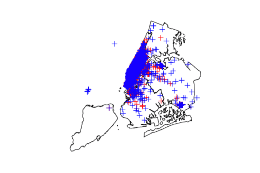
Below are images showing, by 10-minute chunk, where pick ups and drop offs occurred on a map of New York city. Overall, the images show a heavy concentration of rides to and from Manhattan, with only a few extending outside this area. This would suggest, at least during this time frame, that there is a huge potential for successful ride aggregation. (Author’s Note: only one image is included for brevity in the post)
#code prep
setwd("~/kitematic/Via Project")
library(rgdal)
boundaries <- readOGR(dsn = "Borough Boundaries/geo_export_ec8bde98-8133-4640-965d-5a09fec0044b.shp")

boundaries <- spTransform(boundaries, CRS("+proj=longlat +datum=WGS84"))

#1
pickup1 <- subset(monday.700, select = c(pickup_longitude, pickup_latitude))
dropoff1<- subset(monday.700, select = c(dropoff_longitude, dropoff_latitude))

pickup1sp <- SpatialPoints(pickup1)
dropoff1sp <- SpatialPoints(dropoff1)

#2
pickup2 <- subset(monday.710, select = c(pickup_longitude, pickup_latitude))
dropoff2<- subset(monday.710, select = c(dropoff_longitude, dropoff_latitude))

pickup2sp <- SpatialPoints(pickup2)
dropoff2sp <- SpatialPoints(dropoff2)

#3
pickup3 <- subset(monday.720, select = c(pickup_longitude, pickup_latitude))
dropoff3<- subset(monday.720, select = c(dropoff_longitude, dropoff_latitude))

pickup3sp <- SpatialPoints(pickup3)
dropoff3sp <- SpatialPoints(dropoff3)

#4
pickup4 <- subset(monday.730, select = c(pickup_longitude, pickup_latitude))
dropoff4<- subset(monday.730, select = c(dropoff_longitude, dropoff_latitude))

pickup4sp <- SpatialPoints(pickup4)
dropoff4sp <- SpatialPoints(dropoff4)

#5
pickup5 <- subset(monday.740, select = c(pickup_longitude, pickup_latitude))
dropoff5 <- subset(monday.740, select = c(dropoff_longitude, dropoff_latitude))

pickup5sp <- SpatialPoints(pickup5)
dropoff5sp <- SpatialPoints(dropoff5)

#6
pickup6 <- subset(monday.750, select = c(pickup_longitude, pickup_latitude))
dropoff6 <- subset(monday.750, select = c(dropoff_longitude, dropoff_latitude))

pickup6sp <- SpatialPoints(pickup6)
dropoff6sp <- SpatialPoints(dropoff6)

plot(boundaries)
plot(pickup1sp, col="red", add=TRUE)

plot(dropoff1sp, col="blue", add=TRUE)